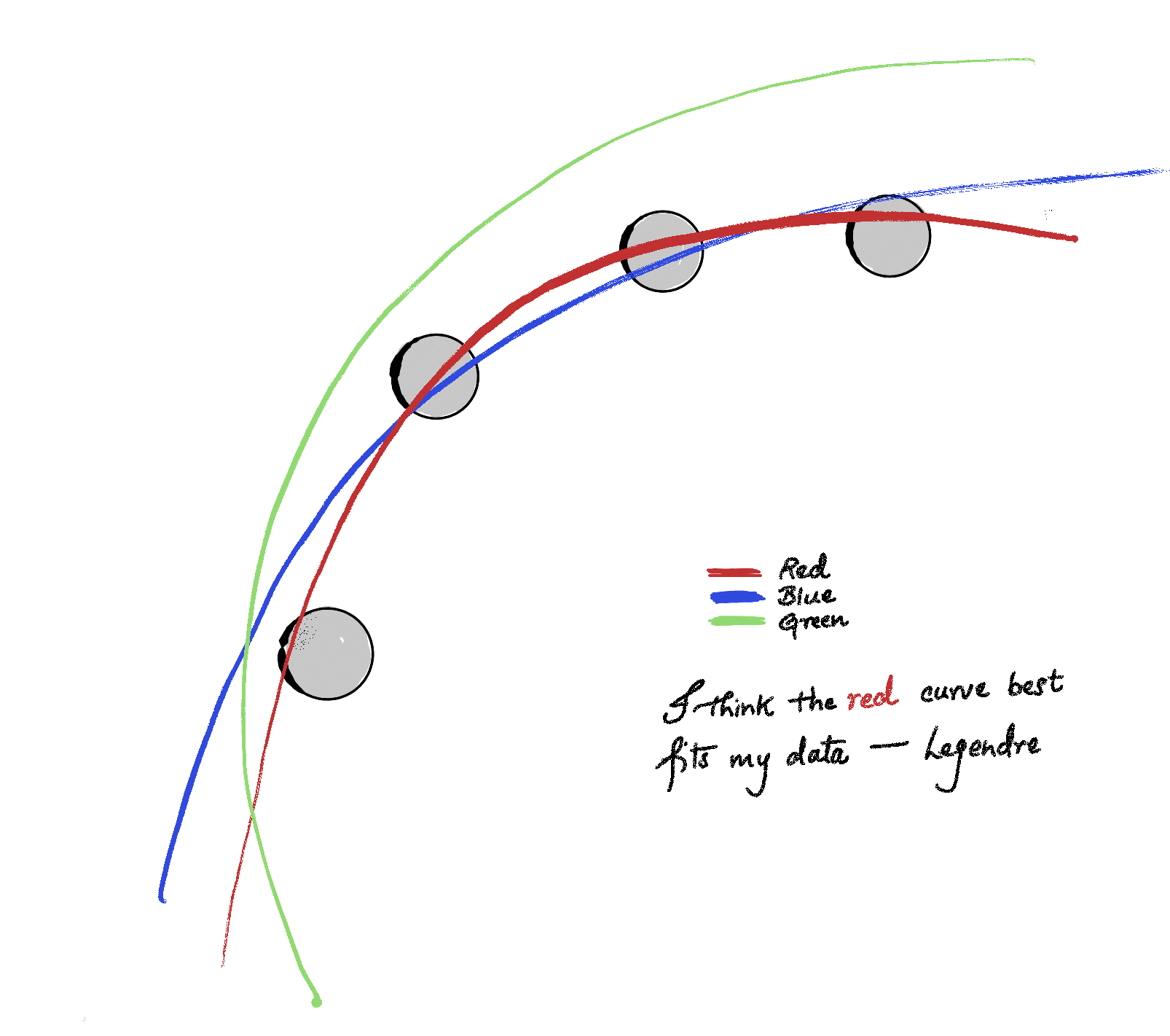
The story begins with making predictions—in prehistoric times they were based on omens, oracles, and divine indication, but the practice of making mathematically sound predictions based on data started with the astronomers of the 18th and 19th centuries who were trying to predict the orbital path of celestial objects. The French mathematician Adrien-Marie Legendre is credited with having first published the formal description of the method of least squares in 1805, as an appendix to his work on the orbits of comets. He was working on a curve-fitting problem— given a set of observations of a comet’s position across several nights, find the parameters for a parabolic path that best fits all the data simultaneously (see Figure 1 ).
Figure 1: Illustration of best-fit orbit.
Since the measurements are noisy and there might not exist a single parabola passing through all the data points simultaneously, Legendre sought to minimize the errors instead: \[\text{minimize } \epsilon_1^2 + \epsilon_2^2 + \cdots ,\] where \(\epsilon_i\) is the error—also called residual—between the observed and predicted position. Why square the residuals? Well, residuals can be both positive and negative, and you don’t want them to cancel each other out. Squaring makes everything positive, yielding a non-negative of the errors. There is a deeper reason than merely measuring positive residuals–namely, the total error (loss) becomes a differentiable function, whose minima can be calculated easily. And there is an even deeper reason from statistics –à la Gauss– which we won’t go into.
Linear Regression
I cannot define regression better than the Merriam-Webster—a functional relationship between two or more correlated variables that is often empirically determined from data and is used especially to predict values of one variable when given values of the others. So when we just add the adjective “linear” and voilà, we get linear regression. A function is linear if it is formed by sums of input variables multiplied by constants. For example, \(f(x) = 2x\) is linear in \(x\). For a multi-variable example take \(f(x, y) = 5x + 3y\). A function like \(f(x)= 3x^2 + 2\) would not be linear (it is quadratic because of the square term).
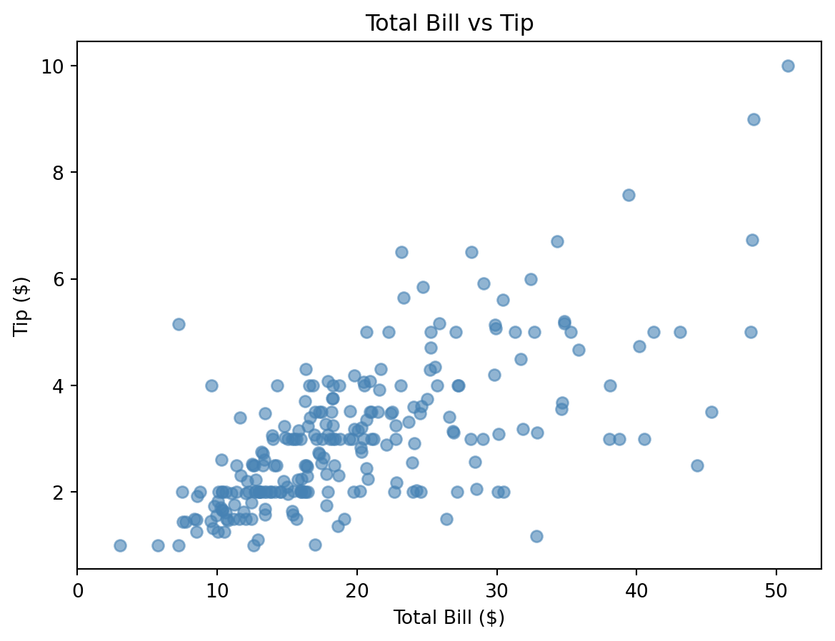
Let’s consider the “tips” dataset from seaborn. In Figure 2 we plot the tip amount against the total bill for the rows in the “tips” dataset. In mathematical terminology, total bill would be called the input and tip amount would be called the output. In statistical and machine learning terminology, total bill would be the predictor/independent variable/explanatory variable/covariate/feature while the tip amount be called the response/dependent variable/outcome/target.
Code
import seaborn as snsimport matplotlib.pyplot as pltdf = sns.load_dataset("tips")plt.figure(figsize=(7, 5))plt.scatter(df["total_bill"], df["tip"], alpha=0.6, color="steelblue")plt.xticks(range(0,51,10))plt.xlabel("Total Bill ($)")plt.ylabel("Tip ($)")plt.title("Total Bill vs Tip")plt.show()
Figure 2: Tip amount vs. Total Bill.
In this example, the goal of linear regression is to draw a line that best fits the data in the scatter plot. From Figure 2 we see that the line should be positive sloped (increasing). In fact, we expect the tips to be roughly proportional to the total bill (higher bills have higher tips, while lower bills have lower tips). But there are outliers, and this is also expected from our experiences–Statistics does not aim for a perfect relationship. To say it more mathematically, it is mathematically impossible for a single line to pass through all the data points. And hence, we are in the situation of Legendre, we restate the goal–we want to minimize the errors.
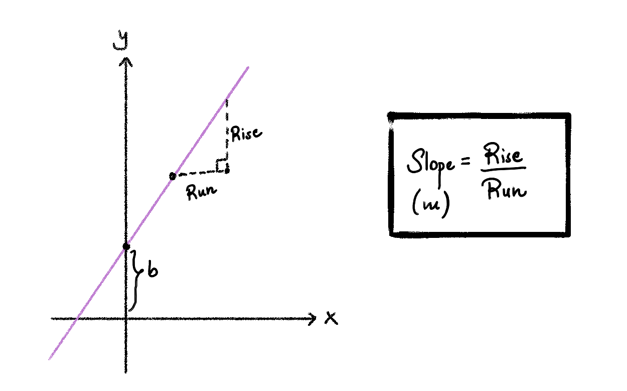
To formalize the problem, first let’s define the family of lines that we could use to fit this data. We know from high-school algebra, that the equation of a line in the plane is given by \(y = mx + b\), where \(m\) is the slope of the line and \(b\) is the y-intercept/vertical intercept (see Figure 3 for the illustration of the equation of a line.)
Figure 3: Illustration of Slope of equation of line.
For the scatter plot from the tips dataset, we can fit various lines in the plane. In Figure 4 you can experiment with various values of \(m\) and \(b\) to find lines that fit the data.
Code
import plotly.io as piopio.renderers.default ="notebook"import plotly.graph_objects as goimport numpy as npimport seaborn as snsdf = sns.load_dataset("tips")x = np.linspace(df["total_bill"].min(), df["total_bill"].max(), 100)m_values = np.arange(0.0, 0.35, 0.05)b_values = np.arange(-0.5, 3.0, 0.5)n_m, n_b =len(m_values), len(b_values)scatter = go.Scatter( x=df["total_bill"], y=df["tip"], mode="markers", marker=dict(color="steelblue", opacity=0.5), name="Data")m_traces = [ go.Scatter(x=x, y=m * x +0.5, mode="lines", line=dict(color="red", width=2), visible=(i ==0), name=f"m={m:.2f}")for i, m inenumerate(m_values)]b_traces = [ go.Scatter(x=x, y=0.15* x + b, mode="lines", line=dict(color="green", width=2), visible=False, name=f"b={b:.1f}")for j, b inenumerate(b_values)]all_traces = [scatter] + m_traces + b_traces# m slider: show m_traces[i], hide all b_tracesm_steps = []for i inrange(n_m): vis = [True] vis += [j == i for j inrange(n_m)] vis += [False] * n_b m_steps.append(dict( method="restyle", args=[{"visible": vis}], label=f"{m_values[i]:.2f}" ))# b slider: show b_traces[j], hide all m_tracesb_steps = []for j inrange(n_b): vis = [True] # scatter always visible vis += [False] * n_m # all m_traces hidden vis += [k == j for k inrange(n_b)] # only b_trace[j] visible b_steps.append(dict( method="restyle", args=[{"visible": vis}], label=f"{b_values[j]:.1f}" ))sliders = [dict( active=0, currentvalue={"prefix": "Slope (m): ", "xanchor": "left"}, pad={"t": 30, "b": 10}, steps=m_steps, x=0, y=0, len=1.0# negative y = below plot ),dict( active=0, currentvalue={"prefix": "Intercept (b): ", "xanchor": "left"}, pad={"t": 30, "b": 10}, steps=b_steps, x=0, y=-0.4, len=1.0# further below )]fig = go.Figure(data=all_traces)fig.update_layout( autosize=True, width=600, height=550, sliders=sliders, title="Total Bill vs Tip", xaxis_title="Total Bill ($)", yaxis_title="Tip ($)", margin=dict(t=50, b=200, l=50, r=50) )fig.show()
Figure 4: Interactive line with slope and intercept sliders
Let \((x_1,y_1), (x_2,y_2), \cdots (x_n,y_n)\) be data points. Let \(y= mx + b\) be an arbitrary line. For a given x, we denote the linear regression prediction by \(\hat{y}:= mx + b\). The residual (error) for a given point \((x_i, y_i)\) is \(y_i - \hat{y}_i = y_i - (mx_i + b)\). It is the vertical distance from the point to the line.
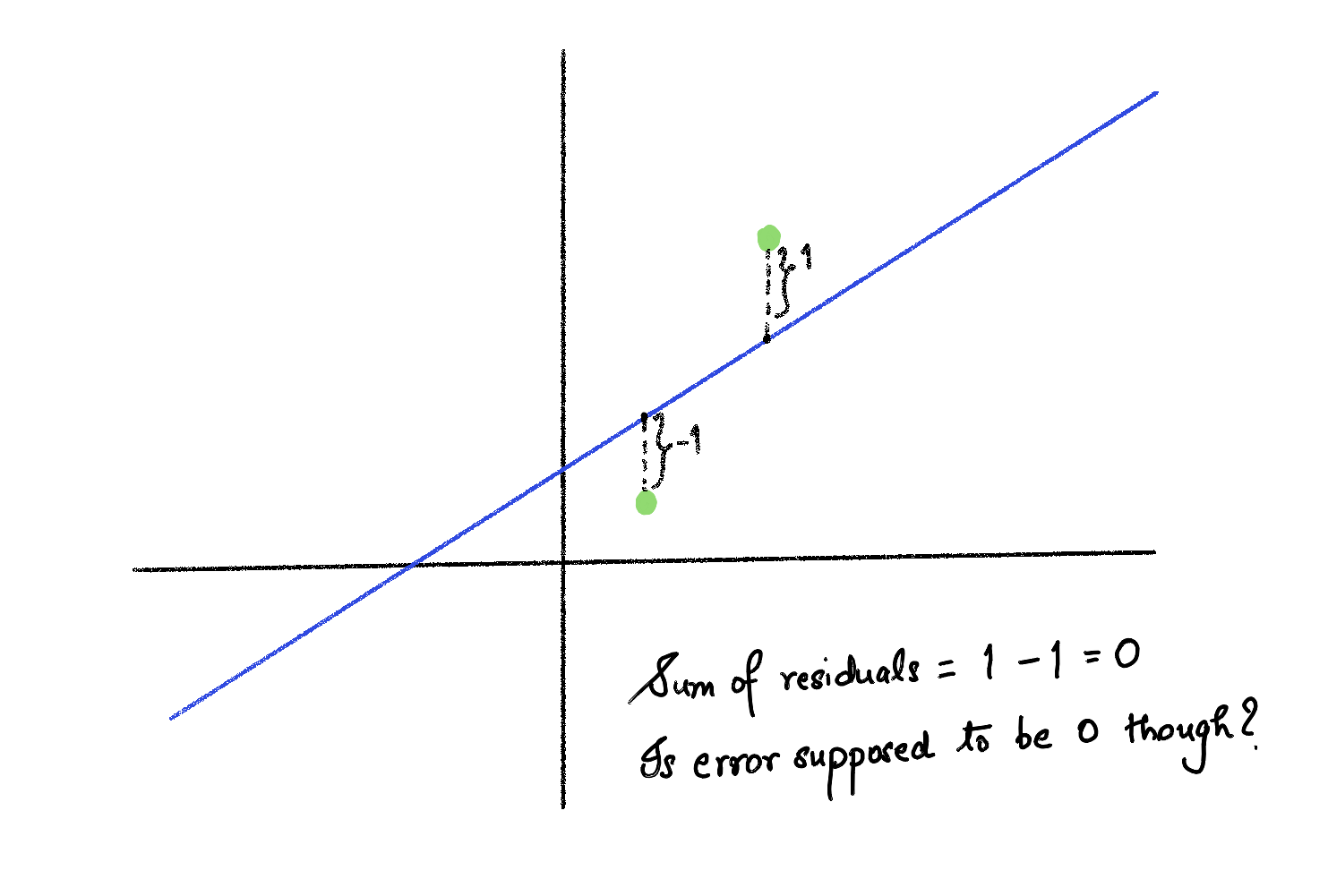
Now we want a single overall measure accounting for all the residuals. Adding the residuals to get the overall error does not work, because some residuals are positive while others are negative, and we don’t want errors to cancel out. For instance, look at Figure 5.
Figure 5: Illustration of residuals cancelling out.
Instead of adding up the residual we add up the squares of the residuals. We call this sum SSR, short for sum of squares of residuals. Note that SSR is 0 if and only if the best fit line passes through all the data points. SSR is large if the residuals are large on average, and SSR is small if the residuals are small on average. We have
our goal is: \[ \text{Find the best m and b to minimize } SSR\]
So now we have a formalized goal—we want to find the line that minimizes the SSR. This line is called the best-fit line. In Figure 6 you can tinker with the \(m\) and the \(b\) values to find a line that minimizes the SSR.
Code
import plotly.io as piopio.renderers.default ="notebook"import plotly.graph_objects as goimport numpy as np# 4 fixed pointsx_pts = np.array([1, 2, 3, 4])y_pts = np.array([1.5, 2.5, 2.0, 3.5])labels = ["(x₁,y₁)", "(x₂,y₂)", "(x₃,y₃)", "(x₄,y₄)"]x_line = np.linspace(0, 5, 100)m_values = np.round(np.arange(0.0, 1.1, 0.1), 2)b_values = np.round(np.arange(-1.0, 3.25, 0.25), 2)n_m, n_b =len(m_values), len(b_values)fixed_b =0.5# b held fixed when m slider movesfixed_m =0.5# m held fixed when b slider movesdef compute_ssr(m, b):return np.sum((y_pts - (m * x_pts + b))**2)def residual_trace(m, b): xs, ys = [], []for xi, yi inzip(x_pts, y_pts): xs += [xi, xi, None] ys += [yi, m * xi + b, None]return go.Scatter(x=xs, y=ys, mode="lines", line=dict(color="orange", width=2, dash="dash"), showlegend=False, visible=False)def ssr_annotation(m, b): ssr = compute_ssr(m, b)returndict( x=0.02, y=0.95, xref="paper", yref="paper", text=f"<b>SSR = Σ(yᵢ - ŷᵢ)² = {ssr:.3f}</b>", showarrow=False, font=dict(size=13), bgcolor="rgba(255,255,200,0.8)", bordercolor="orange", borderwidth=1 )# Tracesscatter = go.Scatter( x=x_pts, y=y_pts, mode="markers+text", text=labels, textposition="top center", marker=dict(color="steelblue", size=12), showlegend=False)# m slider traces (b fixed)m_line_traces = [ go.Scatter(x=x_line, y=m * x_line + fixed_b, mode="lines", line=dict(color="red", width=2), visible=(i ==0), showlegend=False)for i, m inenumerate(m_values)]m_res_traces = [residual_trace(m, fixed_b) for m in m_values]m_res_traces[0].visible =True# b slider traces (m fixed)b_line_traces = [ go.Scatter(x=x_line, y=fixed_m * x_line + b, mode="lines", line=dict(color="red", width=2), visible=False, showlegend=False)for b in b_values]b_res_traces = [residual_trace(fixed_m, b) for b in b_values]all_traces = [scatter] + m_line_traces + m_res_traces + b_line_traces + b_res_traces# m slider stepsm_steps = []for i, m inenumerate(m_values): vis = ([True]+ [j == i for j inrange(n_m)]+ [j == i for j inrange(n_m)]+ [False] * n_b+ [False] * n_b) m_steps.append(dict( method="update", args=[{"visible": vis}, {"annotations": [ssr_annotation(m, fixed_b)]}], label=f"{m:.1f}" ))# b slider stepsb_steps = []for j, b inenumerate(b_values): vis = ([True]+ [False] * n_m+ [False] * n_m+ [k == j for k inrange(n_b)]+ [k == j for k inrange(n_b)]) b_steps.append(dict( method="update", args=[{"visible": vis}, {"annotations": [ssr_annotation(fixed_m, b)]}], label=f"{b:.2f}" ))sliders = [dict(active=0, currentvalue={"prefix": "Slope (m): ", "xanchor": "left"}, pad={"t": 30, "b": 10}, steps=m_steps, x=0, y=0, len=1.0),dict(active=0, currentvalue={"prefix": "Intercept (b): ", "xanchor": "left"}, pad={"t": 30, "b": 10}, steps=b_steps, x=0, y=-0.45, len=1.0)]fig = go.Figure(data=all_traces)fig.update_layout( sliders=sliders, annotations=[ssr_annotation(m_values[0], fixed_b)], title="Residuals and Sum of Squared Residuals", xaxis_title="x", yaxis_title="y", autosize=True, height=550, width=600, margin=dict(t=50, b=200, l=50, r=50))fig.show()
Figure 6: Residuals and sum of squared residuals
After tinkering for a while, you realize, “Hey! There should be a mathematical way to find the best \(m\) and \(b\), right?”. And there is! You can try it:
TipExercise
Let \((x_1,y_1), (x_2,y_2), \cdots, (x_n,y_n)\) be the data points. The best \(m^*\) and \(b^*\) that minimize SSR are given by
where \(\bar{x} = \frac{x_1+x_2+\cdots+x_n}{n}\) and \(\bar{y} = \frac{y_1+y_2+\cdots+y_n}{n}\).
Trust me. You just need algebra for this.
Note that \(b^*\) ensures the best-fit line always passes through the point \((\bar{x}, \bar{y})\).
If you know covariance and variance, \(m^*\) is simply \(\frac{\text{Cov}(x,y)}{\text{Var}(x)}\).
In Python there are libaries that find the best-fit line for us. We will get into it soon, but before that just a little bit more theory.
Measuring the goodness of fit (R- squared)
For a given set of data points, we know how to find the best-fit line (linear regression), and now we want a single number that tells us how well the model fits this data.
TipQuestion
But didn’t the SSR already do that? High SSR is bad and small SSR is good? Not quite.
If I tell you SSR = 50, you don’t know if that’s a great fit or a terrible one. It depends entirely on the scale of your data. If your target values are in the range [0, 1], that’s catastrophic. If they’re in the millions, it’s essentially perfect.
The \(R^2\) measure we discuss below gives us a normalized measure of how good a linear regression model fits the data, in other words, how much of the variance is accounted for by the linear regression model.
To derive \(R^2\), we will compare two models—a base model which is just a constant (null model) and our regression model. \(R^2\) essentially measures how much of an improvement the linear regression model makes over the null model. Given data points \(y_1, y_2, \cdots y_n\) (we are taking the target values), the expected value (average) of the y values is \[ \bar{y} = \frac{y_1 + y_2 + \cdots y_n}{n}.\] The null model’s prediction for any arbitrary input x is just \(\bar{y}\). In other words, we are saying, “We are not going to claim any relation between the dependent variable and the independent variable”. Irrespective of the input, we make the constant prediction: \(\bar{y}\). On the other hand, for the linear regression model, we will use a best-fit line to model our data. See Figure 7 for a comparison of the residuals for the null model and the linear regression models (tips dataset).
For the null model, we will call the sum of the squares of the residuals SST (total sum of squares). We have \[ \text{SST} = \sum_{i=1}^{n} (y_i - \bar{y})^2 \]
For the linear regression model, we have \[ \text{SSR} = \sum_{i=1}^{n} (y_i - \hat{y}_i)^2 \] where \(\hat{y}_i\) is \(m^*x_i + b^*\): the prediction for \(x_i\) from the best-fit line.
Now consider the difference: \[ \text{SST} - \text{SSR}\]
Well, why not just take this absolute difference as our measure? There are a few reasons for this - This is scale/unit dependent. For instance, if I use cents instead of dollars, \(\text{SST} - \text{SSR}\) will be 10000 times the one I get for dollars. - We cannot interpret the difference easily— What does \(\text{SST} - \text{SSR} = 20\) mean?
Instead we want: what fraction of SST the regression model accounts for. Also, \(R^2\) fixes both the above issues. Hence, we have
Note that \(R^2\) is a value in \((-\infty,1]\). A value of 0 means the regression model is no better than the null model. It means SSR = SST, i.e. the regression explains none of the variance. A value of 1 means that the best-fit line passes through all the data points.
We can see some examples of the different \(R^2\) values in Figure 8.